How foundation audio models and Audio LLMs bridge the gap between acoustic similarity and perceptual relevance
TL;DR
- Acoustic similarity ≠ perceptual relevance. Two tracks can share timbre and tempo yet serve opposite listening contexts.
- Embedding models measure sound; Audio LLMs reason about context. Foundation models (MusicFM, CLAP, MuQ-MuLan) provide fast vector retrieval. Audio LLMs (Qwen2-Audio, Music Flamingo, Qwen3-Omni, LTU) add compositional reasoning and explainability.
- The future of music recommendation is fast retrieval + slow reasoning. A hybrid pipeline retrieves candidates via embeddings, captions them offline, and reranks with an LLM judge — then feeds those judgments back as hard negatives to strengthen the embedding space.
Introduction

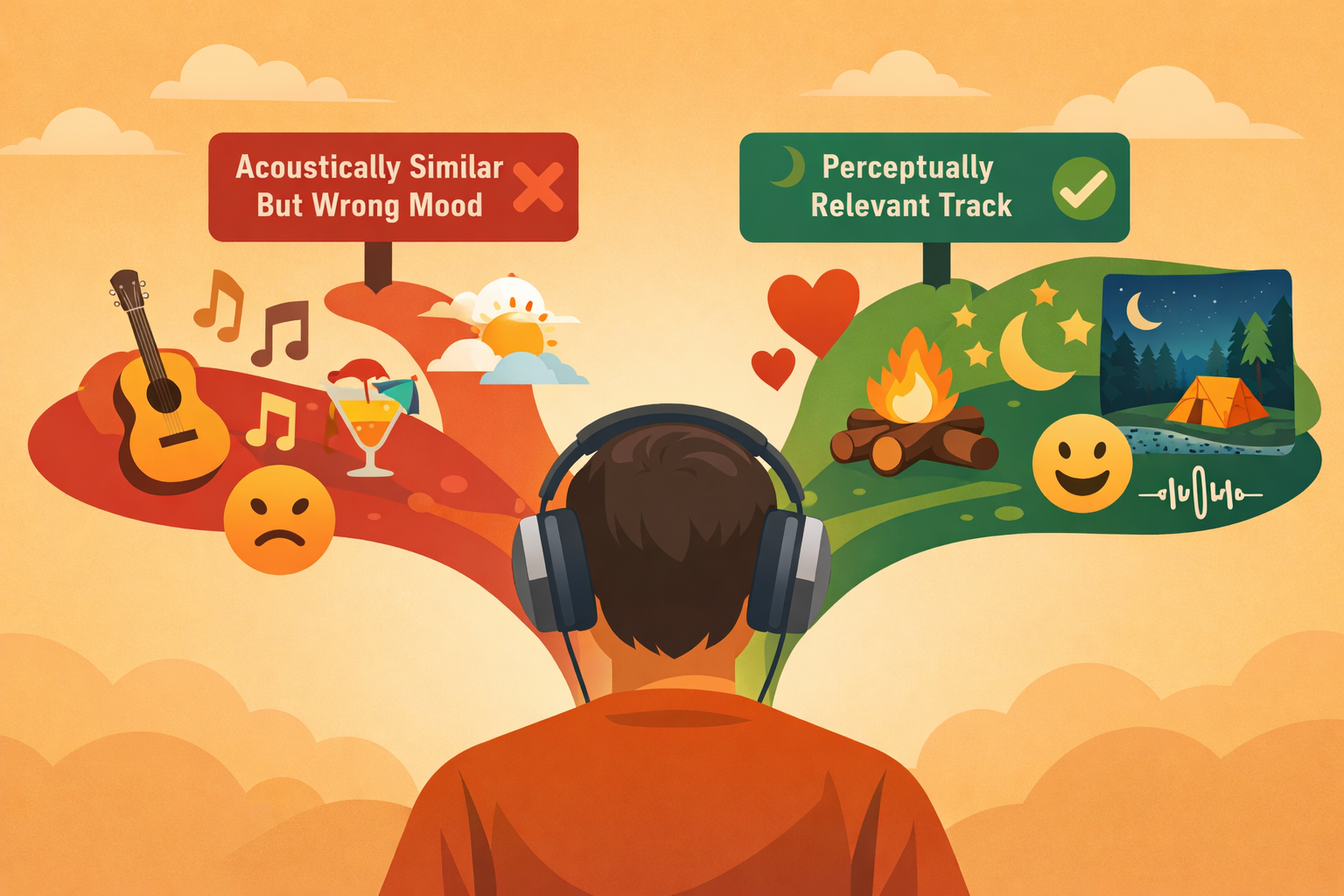
Imagine you’re listening to a melancholic indie folk track with soft acoustic guitar and hushed vocals. You want more music like this. Your streaming service suggests another track — same genre tag, similar tempo, comparable acoustic features. But when you hit play, something feels off. The new track is upbeat and energetic, completely mismatched to your contemplative mood.
This disconnect reveals a fundamental challenge in music recommendation: acoustic similarity doesn’t equal perceptual relevance.
Traditional content-based systems excel at measuring what music sounds like — tempo, timbre, spectral features — but struggle to capture what it means and why it matters to listeners in specific contexts. Music similarity is inherently multi-dimensional and context-dependent. Two tracks might share identical instrumentation and tempo yet serve completely different purposes: one for intense workouts, another for late-night studying.
Human perception of music relevance is dynamic, shaped by listening intent, emotional state, and cultural context — factors that often contradict simple distance metrics in embedding spaces. This mismatch is the semantic gap: the disconnect between measurable acoustic similarity and human-perceived contextual relevance.
Relevance is not a static property of a track pair. It is a function conditioned on listener intent.
Audio Language Models (Audio LLMs) address this gap by combining audio encoders with large language models to enable semantic reasoning about music. They bridge acoustic features and human-interpretable meaning, transforming how we assess music relevance, generate recommendations, and explain why tracks matter to specific listeners.
This article explores:
- How audio signals are transformed into ML-models-friendly representations.
- How audio foundation (trained in unsupervised fashion) models (MusicFM, CLAP, MuQ-MuLan) provide fast semantic retrieval — and where they fall short.
- How Audio LLMs add reasoning, explainability, and contextual judgment.
- How both approaches can support each other, with practical examples using Qwen3-Omni captioning and MuQ embeddings.
The Semantic Gap: Three Dimensions of Music Similarity
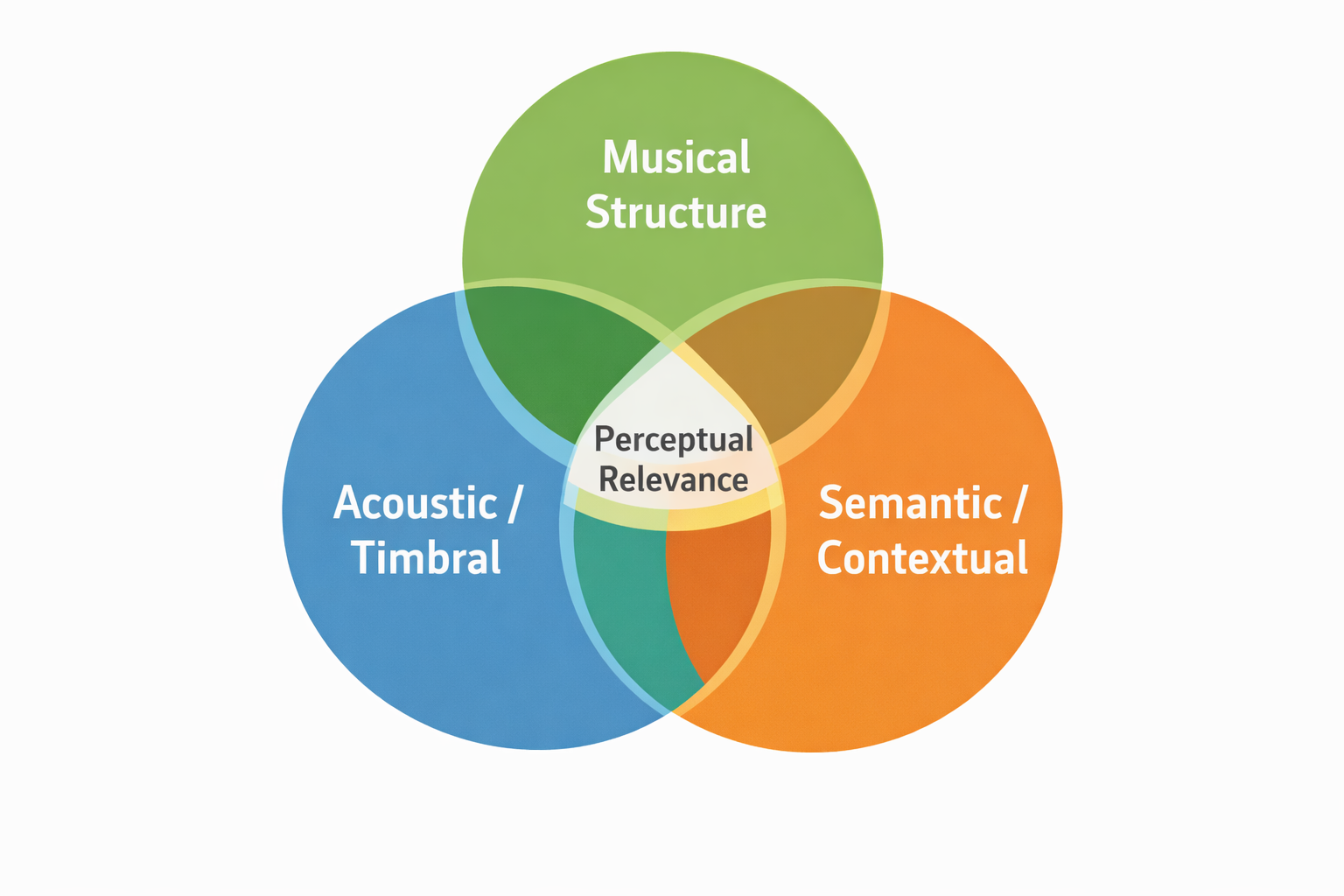
Music similarity exists across three overlapping but distinct dimensions:
Acoustic / Timbral Similarity
The physical, low-level characteristics of sound: spectral envelope, timbre, tempo, texture, and instrumentation. This is the what of music. Two tracks with similar drum patterns, guitar tones, and vocal textures score high here. Modern foundation models like MusicFM excel at learning these representations through masked audio modeling on mel spectrograms.
Musical Structure
The compositional, higher-level elements: genre conventions, harmonic progressions, melody (fundamental-frequency contour), tonality, rhythmic patterns, and song form. This is the how — how sounds are organized in time. A blues song and a jazz standard might share chord progressions and swing rhythms despite different timbres. Many studies report that rhythm and melody dominate human similarity judgments more than timbre alone — yet most embedding models still overemphasize timbral cues.
Semantic / Contextual Similarity
The why of music — mood, emotional impact, cultural associations, functional usage (study, gym, meditation), and genre. Two songs might sound completely different acoustically yet both evoke nostalgia or work perfectly for a rainy Sunday morning. This dimension is language-grounded and requires reasoning about human experience.
Perceptual relevance emerges at the intersection of all three.
The fundamental challenge: most models capture only one or two dimensions. Embedding models typically collapse everything into a single vector and apply cosine similarity — losing contextual nuance. True relevance assessment requires reasoning across all three simultaneously.
From Waveforms to Embeddings: The Audio Representation Pipeline
Before any model can reason about music, the raw audio signal must be transformed into a structured representation. This section traces the pipeline from pressure waves to the discrete or continuous tokens that foundation models consume.
Raw Waveform
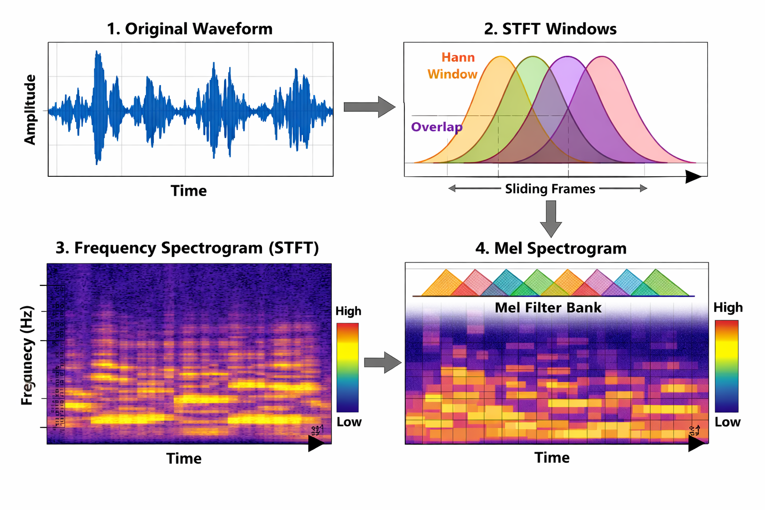
Music exists as continuous pressure waves $x(t) \in \mathbb{R}$. Digital audio samples these at $f_s$ (typically 44.1 kHz), yielding a discrete waveform $x[n]$. Raw waveforms are extremely high-dimensional, non-stationary, poorly aligned with human perception, and over-redundant for downstream modelling.
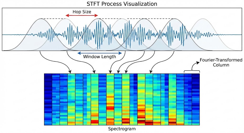
Short-Time Fourier Transform (STFT)
Music is non-stationary — its frequency content changes over time. The standard Fourier Transform assumes stationarity, so we apply it locally via overlapping sliding windows:
$$X(m, \omega) = \sum\_{n=-\infty}^{\infty} x[n] \, w[n - m] \, e^{-j\omega n}$$where $w[\cdot]$ is a window function (e.g. Hann), $m$ indexes time frames, and $\omega$ indexes frequency. Taking the magnitude $|X(m, \omega)|$ yields the spectrogram — a 2D time–frequency representation.
Mel-Scale Transformation
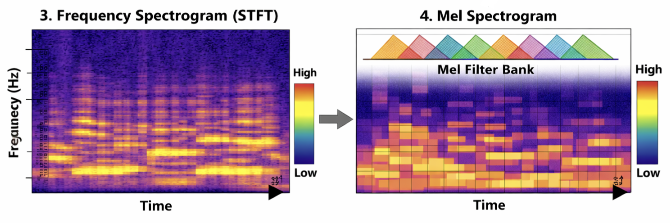
Human pitch perception is approximately logarithmic: we easily distinguish 100 Hz from 200 Hz, but not 10,100 Hz from 10,200 Hz. The Mel scale warps frequency to match this perceptual nonlinearity:
$$\text{mel}(f) = 2595 \log\_{10}\!\left(1 + \frac{f}{700}\right)$$We apply a triangular mel filterbank:
$$M(m, k) = \sum\_{\omega} H\_k(\omega)\,|X(m, \omega)|^2$$where $H_k(\omega)$ are triangular mel filters and $k$ indexes mel bins. Finally, log compression converts to decibels:
$$S(m, k) = \log\!\bigl(M(m, k) + \epsilon\bigr)$$This yields the log-mel spectrogram. Without log compression, loud peaks (e.g. drum hits) would dominate, making subtle harmonics numerically invisible to the model. The resulting 2D representation (time × mel-frequency) encodes pitch, harmonics, rhythm, and timbre in a neural-friendly format.
We will not go to further details, but if you want to understand audio signal representations in more details:
For a detailed treatment of audio signal representation (in the speech context, but broadly applicable), see: https://dukan.dev/posts/speech/
From Spectrograms to Tokens
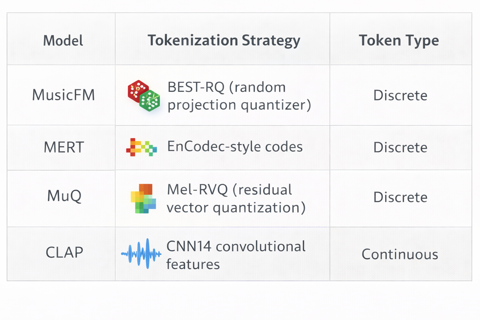
Modern foundation models rarely operate on raw spectrogram pixels. Instead, they convert spectrograms into discrete or continuous token sequences:
This is where we transition from pure signal processing to representation learning. Now lets dive into details of these models and understand their limitations.
Foundation Models and Their Limitations
Lets discuss one of the most popular foundation models, which form the backbone of modern music retrieval. Each advances the state of the art in a different dimension — but all share a critical structural limitation. We discuss their architectures, strengths, and what they cannot do.
MusicFM: Self-Supervised Acoustic Representations
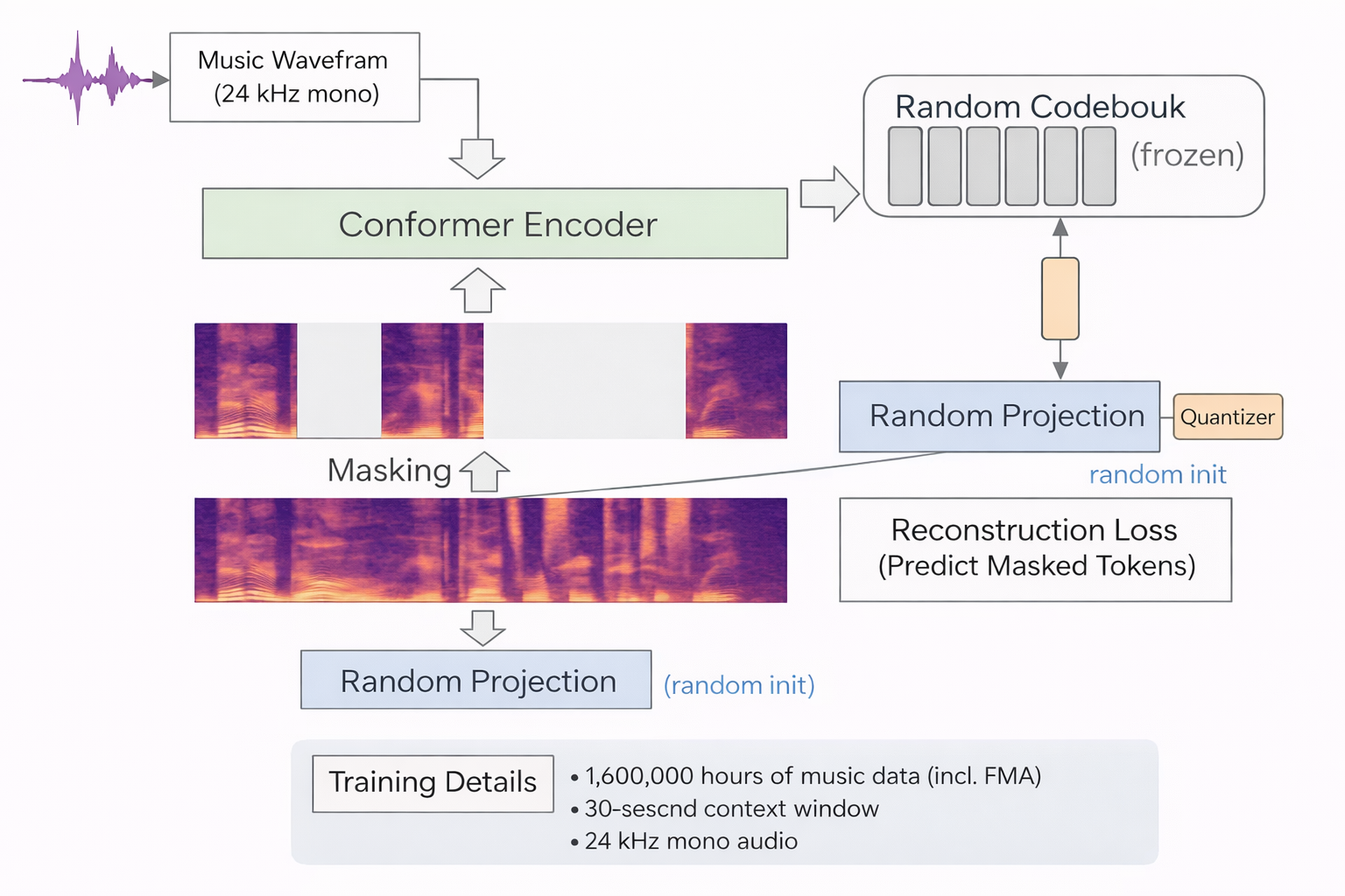
MusicFM applies the masked language modeling paradigm (à la BERT) to music audio. The training recipe:
- Tokenize: Convert mel-spectrogram frames into discrete units via a random-projection quantizer (BEST-RQ). A frozen random projection maps mel frames to a latent space, which is then quantized against a random codebook.
- Mask: Randomly mask a large fraction of tokens (~75%).
- Predict: Train a Conformer (yes – ASR) encoder to reconstruct masked tokens from surrounding context
- Scale: Train on 160k hours of music data (including the Free Music Archive) at 24 kHz mono, with a 30-second context window.
The model learns deep acoustic representations — timbre, rhythm, instrumentation, spectral co-occurrence patterns — that transfer effectively across MIR tasks (tagging, genre classification, instrument recognition).
What MusicFM captures:
- Spectral pattern co-occurrence
- Timbral texture clustering
- Rhythmic and harmonic statistical alignment
What MusicFM does not model:
- Why certain musical features produce specific emotional effects
- How listener intent modulates relevance
- How context transforms similarity judgments
Structure, but no meaning. MusicFM knows what sounds co-occur, not what they mean.
CLAP: Contrastive Language–Audio Alignment
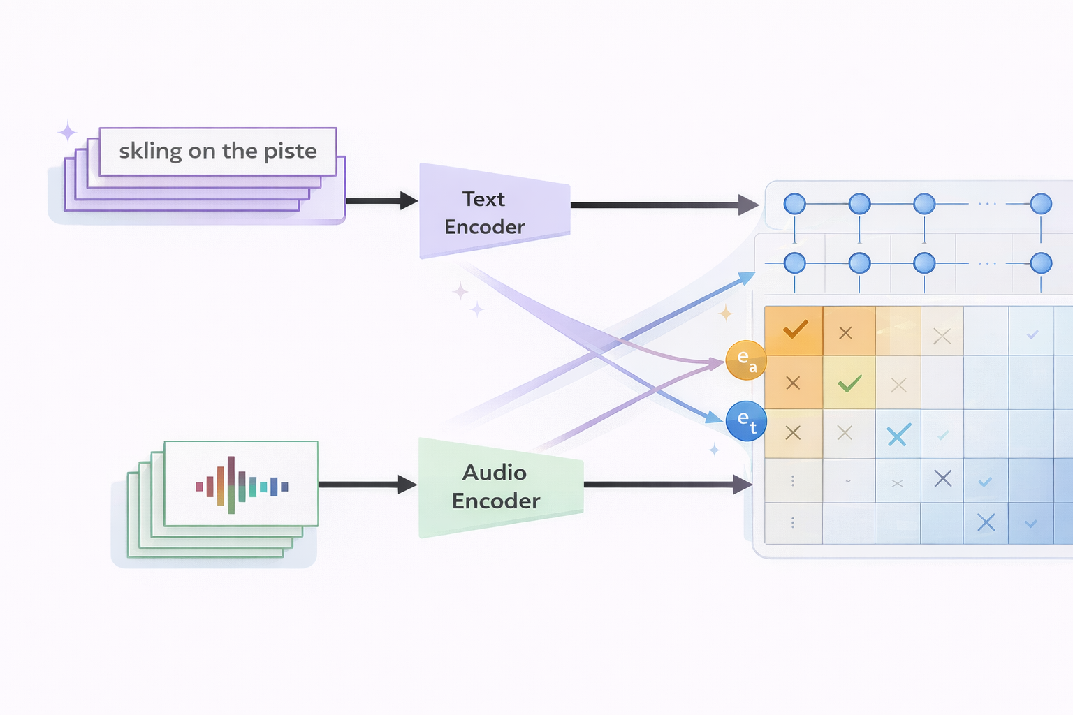
CLAP (Contrastive Language-Audio Pretraining) introduces language supervision by training dual encoders to align audio and text in a shared embedding space. It is the same idea that is used for text-image alignment CLIP models. The objective is the symmetric InfoNCE loss:
$$\mathcal{L}\_{\text{InfoNCE}} = -\frac{1}{2N}\sum\_{i=1}^{N}\left[\log\frac{\exp(\mathbf{e}\_{a\_i}^\top \mathbf{e}\_{t\_i}/\tau)}{\sum\_{j=1}^{N}\exp(\mathbf{e}\_{a\_i}^\top \mathbf{e}\_{t\_j}/\tau)} + \log\frac{\exp(\mathbf{e}\_{t\_i}^\top \mathbf{e}\_{a\_i}/\tau)}{\sum\_{j=1}^{N}\exp(\mathbf{e}\_{t\_i}^\top \mathbf{e}\_{a\_j}/\tau)}\right]$$where $\mathbf{e}_{a_i}$ and $\mathbf{e}_{t_i}$ are the normalized audio and text embeddings for the $i$-th pair, $\tau$ is a learned temperature, and $N$ is the batch size. The loss symmetrically maximizes audio→text and text→audio retrieval within a batch.
This enables:
- Zero-shot classification — retrieve the best-matching text label for unseen audio.
- Cross-modal retrieval — find audio given a text query, or vice versa.
- Fast inference — a single forward pass + approximate nearest neighbors (ANN).
Limitations: CLAP’s semantics are association-based, not causal. “Upbeat” co-occurs with certain tempo/spectral patterns; “acoustic folk” clusters with specific timbral signatures. CLAP learns correlations between acoustic patterns and text labels, not explanations for why musical elements produce perceived effects. Embeddings are also context-independent — the same track always maps to the same point regardless of who is listening or why. Also it is not very suitable for musical tracks comparisons.
Model can be found at: https://huggingface.co/laion/clap-htsat-fused
MuQ-MuLan: Music-Specialized Joint Embeddings
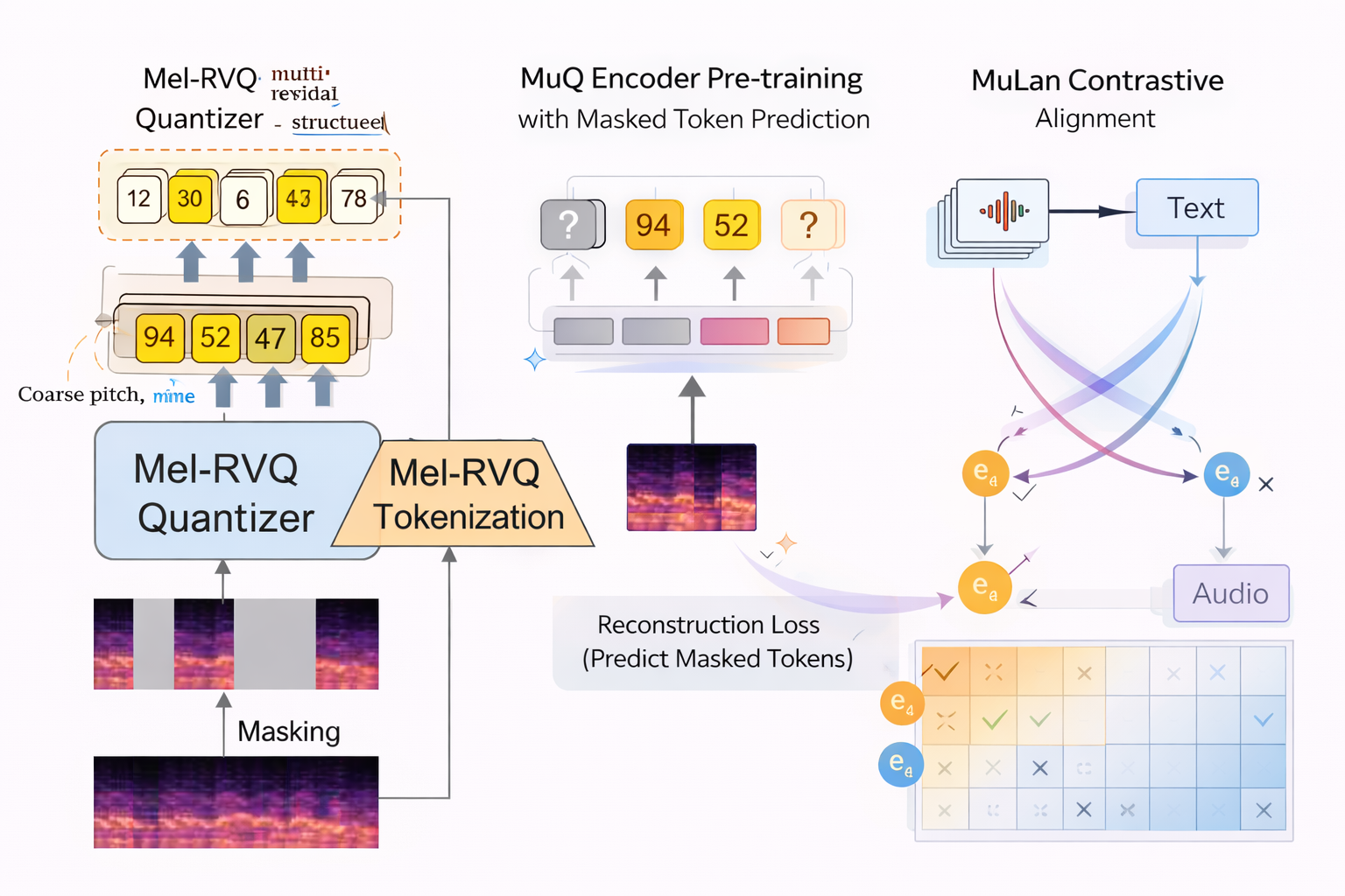
Generic audio encoders (trained on speech and environmental sounds) underperform on music because music has uniquely rich structure — overlapping harmonics, complex rhythmic patterns, tonal hierarchy. MuQ addresses this with a music-specific tokenizer: Mel Residual Vector Quantization (Mel-RVQ).
Mel-RVQ works hierarchically (can think of this idea as similar to gradient boosting algorithms idea of the residuals correction). The first codebook captures coarse spectral structure (pitch, energy). Each subsequent codebook encodes the residual — the difference between the original and the reconstruction so far — capturing progressively finer detail (timbre, harmonics, production texture). This mirrors how music itself is hierarchically structured.
After tokenization, MuQ trains a Transformer encoder via masked token prediction (similar to MusicFM, but with music-aware targets). The resulting representations are then aligned with text via contrastive learning in the MuLan stage, producing a joint music–text embedding space.
MuQ-MuLan currently represents the strongest open music-aware joint embedding backbone, outperforming both MusicFM and CLAP on music retrieval and similarity benchmarks.
Model can be found at: https://huggingface.co/OpenMuQ/MuQ-MuLan-large
The Shared Limitation: Static Cosine Similarity
All three models share a structural assumption, where similarity between items is solely defined by:
$$\text{Similarity}(A, B) = \cos\bigl(\Phi(A), \Phi(B)\bigr) = \frac{\Phi(A) \cdot \Phi(B)}{\|\Phi(A)\| \, \|\Phi(B)\|}$$where $\Phi$ is the encoder. This formulation is:
- Context-free: the same pair always gets the same score regardless of intent.
- Dimension-collapsing: timbre, rhythm, melody, mood, and production are flattened into one number.
- Non-compositional: no mechanism to weight dimensions differently per query.
Large listening studies confirm that human similarity ratings are more complex than cosine distance in any embedding space. Perception is dynamic — listeners weight elements differently depending on task. Rhythm and melody can dominate timbre. The same pair can be “similar” for a workout playlist but “dissimilar” for study music. Also the embedding representation needs to be disentangled to emphasize different similarity aspects, which is quite important for relevance ranking tasks.
This is the semantic gap: the distance between what models measure (acoustic/structural cues) and what humans experience (contextual meaning, emotional impact, functional relevance). This gap cannot be closed by better embeddings alone. Closing it requires models that can reason and understand about music, not just embed it.
Perceptually-Aligned Similarity: An Intermediate Step
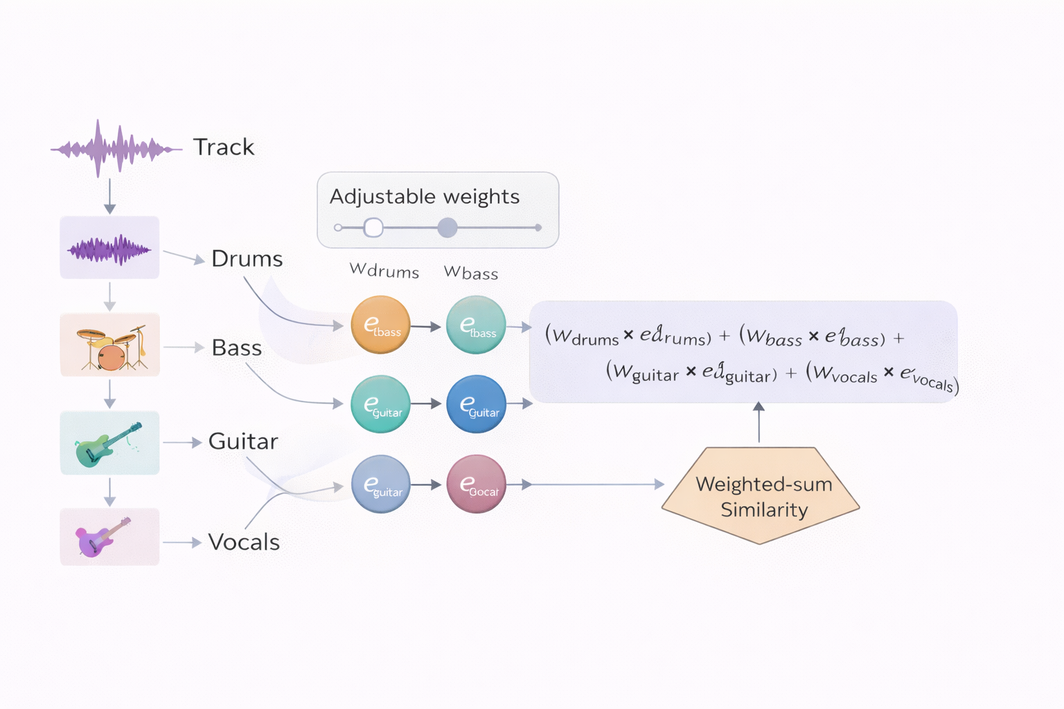
One approach to improve agreement with human judgments is instrument-aware similarity:
$$\text{sim}(A, B) = \sum\_{k} w\_k \cdot \cos\bigl(\phi(A^{(k)}), \phi(B^{(k)})\bigr)$$where $A^{(k)}$ is the $k$-th stem (drums, bass, vocals, etc.) of track $A$, and $w_k$ are learned weights. This yields interpretable, per-instrument similarity scores and better alignment with human ratings. Also using MuQ-Mulan per-instrument embeddings also showed a good correlation between human and embedding distance judgements of similarity.
However, these per-instrument weights $w_k$ are typically fixed after training. Also this instrument disentanglement still does not give too much information about the sound semantics and purpose. Human weighting is context-dependent: “for rhythm similarity, weight drums more; for mood similarity, weight harmony more.” This motivates the need for models that can dynamically adjust — i.e., Audio LLMs.
Audio Language Models: Adding Reasoning
Why Audio LLMs?
Foundation embedding models answer questions like “how similar do these two tracks sound?” Audio LLMs answer fundamentally different questions:
- “Which audio is semantically similar to this anchor, and why?”
- “Which track is more relevant for a user in context C?”
- “What is the mood, meaning, and cultural context of this music?”
- “What is this song about? What is the mood? Is it suitable for training?”
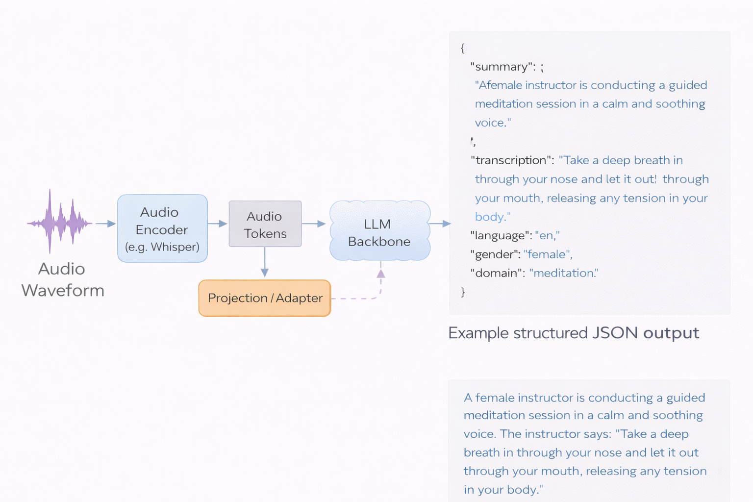
Audio LLMs follow a perception-to-language pattern:
- An audio encoder (e.g. Whisper, CNN14) transforms audio into a token sequence.
- Projection/adapter layers map audio tokens into the LLM embedding space.
- The LLM backbone performs reasoning and text generation conditioned on audio tokens + text prompt.
They bring world knowledge, compositional reasoning, and natural language explanations. Crucially, Audio LLMs augment rather than replace embedding models: embeddings remain the backbone for fast retrieval; LLMs operate on small candidate sets or offline as the inference speed of the LLM is slow and resources-hungry for many online deployments.
Model Landscape
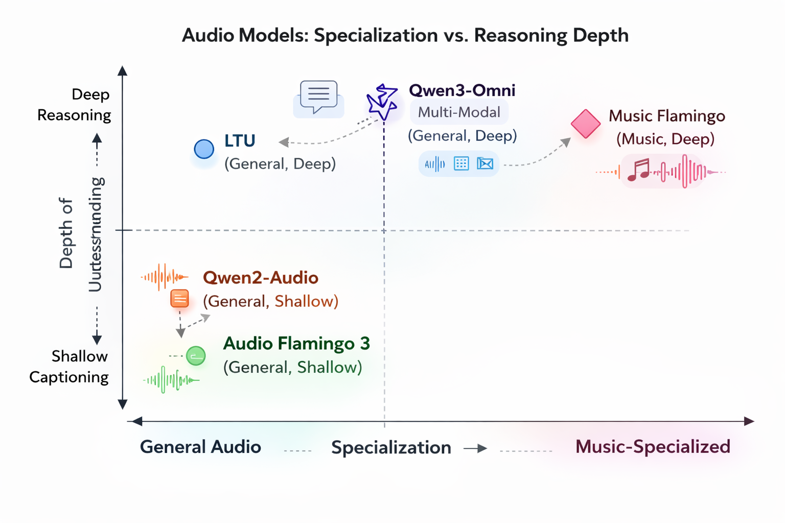
| Model | Audio Encoder | LLM Backbone | Music Focus | Max Audio | Key Strength | Paper |
|---|---|---|---|---|---|---|
| Qwen2-Audio | Whisper-style frontend | Qwen2 (7B) | Medium | ~30s | Stable instruction-following; structured outputs | Qwen2-Audio Technical Report (2024) |
| Audio Flamingo 3 | AF-Whisper | Flamingo-style LLM | Medium | Up to ~10 min | Open-source recipe; broad audio understanding | Audio Flamingo 3 (2025) |
| Music Flamingo | AF-Whisper + temporal alignment | Qwen2.5-7B | High | ~20 min | SOTA music benchmarks; music-focused training; CoT reasoning | Music Flamingo (2025) |
| Qwen3-Omni / Omni Captioner | Modality-specific encoders | 30B MoE | Medium / High | 40+ min | Cross-modal reasoning (text/image/audio/video); Thinker–Talker architecture | Qwen3-Omni Technical Report (2025) |
| LTU | Audio Spectrogram Transformer (AST) | LLaMA-based | Low | ~10s | Perception-to-understanding curriculum; strong comparative reasoning | LTU: Listen, Think, Understand (2023) |
| Kimi-Audio | Hybrid: discrete semantic tokens + Whisper-derived acoustic features | Qwen2.5-7B initialized | Medium | Streaming / chunked | Unified understanding + generation; hybrid tokenization | Kimi-Audio (2025) |
Model Selection Cheatsheet
All these models are available for local deployments. There are other models like Kimi-Audio that are also quite strong, and may be even stronger than Qwen Audio, but Qwen is more popular overall. Also models like GPT 5.2 are also capable with multi-modal reasoning, but can be called only through their APIs.
- Scale metadata extraction → Qwen2-Audio — high structural output stability, good for batch JSON captioning.
- Deep musicological analysis → Music Flamingo — trained on 4M+ music samples with MF-Skills and MF-Think (176k CoT examples), GRPO-tuned. Delivers coherent analyses linking harmony, structure, timbre, vocals, and cultural context.
- Pairwise relevance judgments → LTU — trained on OpenAQA-5M (5.6M audio-QA tuples) with perception-to-understanding curriculum. Useful as an oracle/judge.
- Multi-modal reasoning (audio + lyrics + video) → Qwen3-Omni — 30B MoE, 119 text languages, 19 speech languages, cross-modal reasoning.
- General audio reasoning (open-source) → Audio Flamingo 3 — fully open training recipe from NVIDIA.
We won’t deep dive into other details on audio LLMs in this article — this is more suitable for the separate future discussion, where we will try different LLMs for music and audio relevance tasks and analyze these models architectures, their strengths and weaknesses in details.
Relevance Assessment with Audio LLMs
The problem we want to investigate is whether is possible to use audio LLMs as a substitution for human assessors for musical content recommendation relevance quality. Also the idea of using LLMs for this task is a an idea of the creation of ideally guided assessor, that will compare tracks, based on the understanding of production demand. Also these LLMs can help us to caption the whole catalog of the tracks or help to create data for the internal captioner model. In this article we will merely scratch a surface on these capabilities and set possible directions for future experiments.
Assessment Paradigms
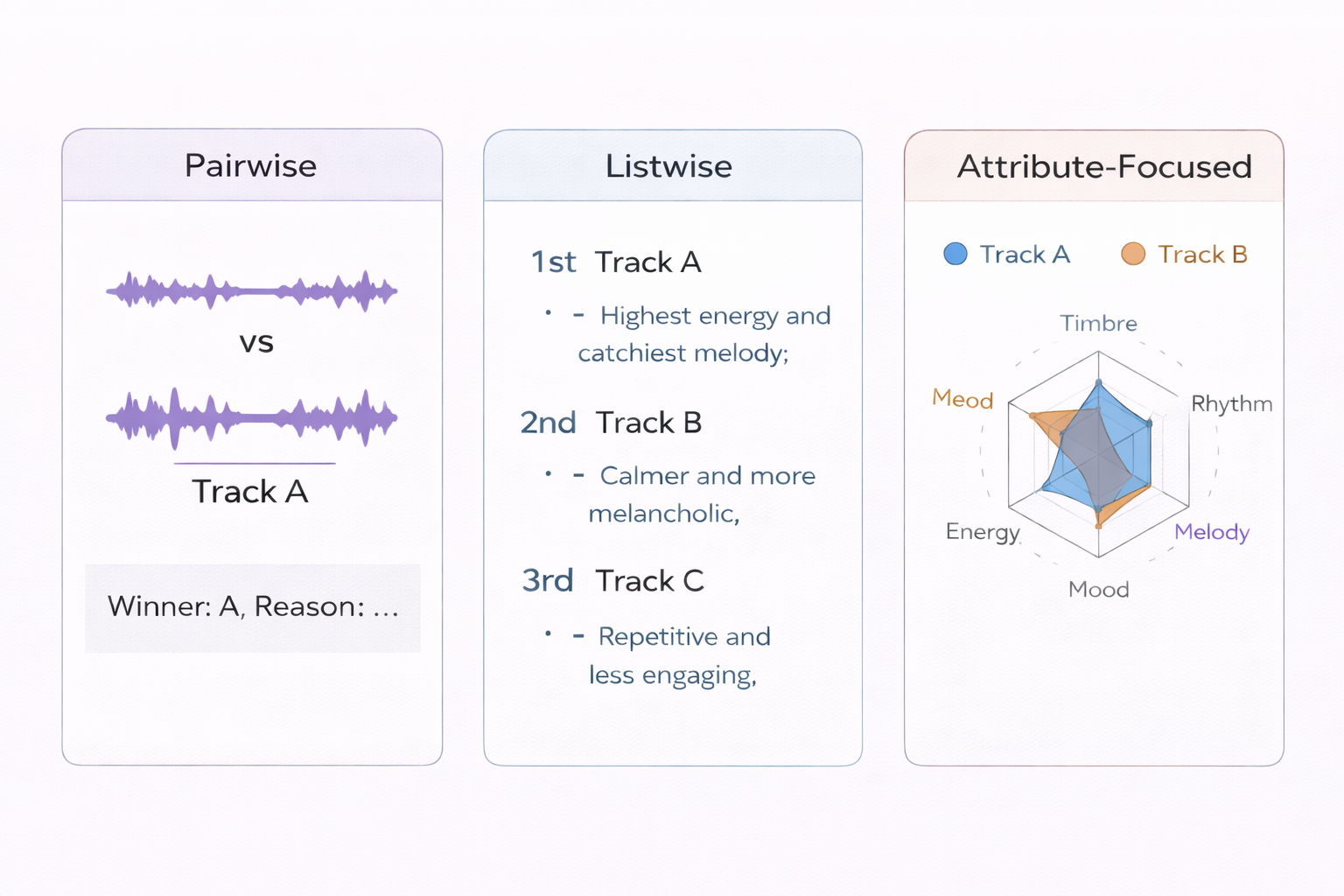
Audio LLMs enable three complementary evaluation paradigms:
- Pairwise comparison — “Given context C, is Track A or Track B more relevant, and why?” Produces a winner + reasoning.
- Listwise ranking — Rank the top-$k$ candidates for a context and explain the ordering.
- Attribute-focused — Compare tracks specifically on rhythm, timbre, mood, energy, etc. Produces dimensional similarity profiles.
Prompting Strategies
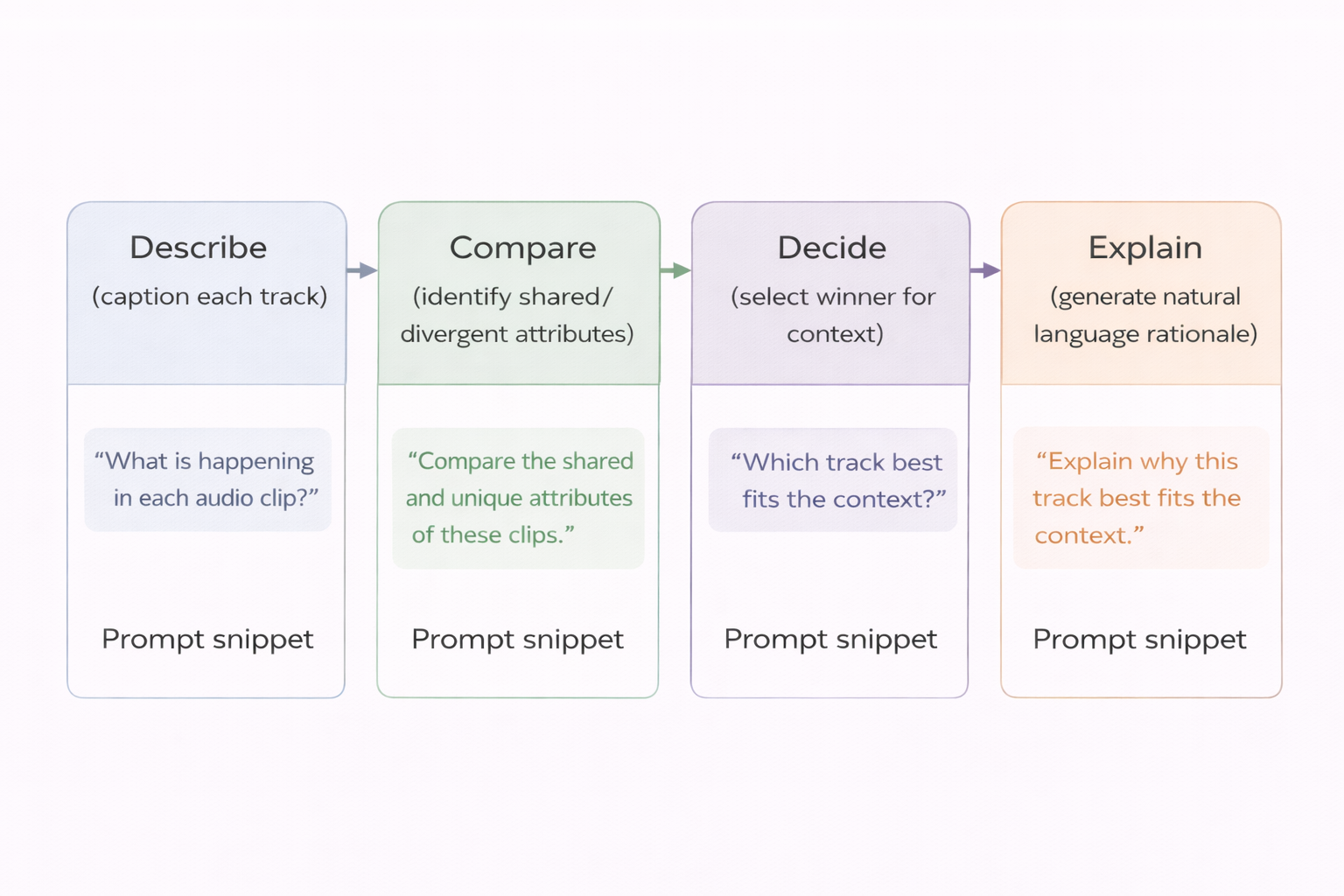
Effective prompting follows a describe → compare → decide → explain pipeline:
- Stepwise reasoning: Force the model to describe each track before comparing, reducing hallucination.
- Role-based instructions: “You are a professional music curator evaluating tracks for a lo-fi study playlist.” – this will help to bias the model towards the required role and task
- Contrastive focus: “Focus on differences in energy, rhythm, and vocal presence.”
- Uncertainty calibration: “If both tracks are equally relevant, say so and explain why.”
Example prompt structure:
Models expect only one music track as input, so we can model 2 tracks input by concatenation of 2 tracks with some pause in-between. If this approach doesn’t work good (based on working with some of the models we encountered difficulties), we always can represent another track as the description (even can at the same time input descriptions for several tracks, by keeping the anchor track as the audio tokens input).
From Judgments to Training Signals: Hard Negative Mining
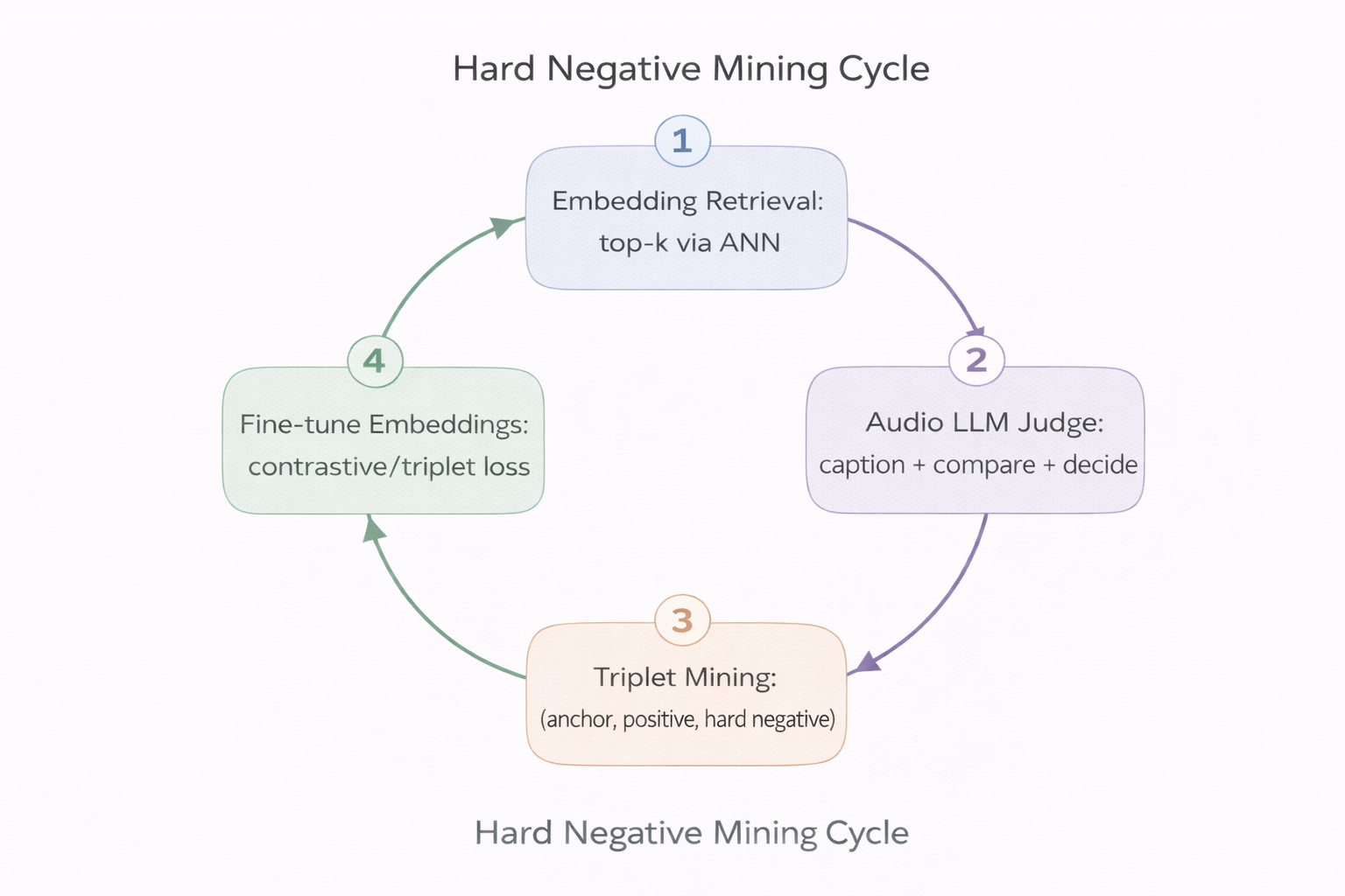
Audio LLM judgments are expensive at inference time. The key insight is to use them offline to generate training signal that strengthens the embedding space itself:
- Retrieve top-$k$ candidates for an anchor track using embedding similarity (fast ANN search).
- Judge candidates with an Audio LLM — caption each track, perform pairwise comparison, produce relevance scores with explanations.
- Mine triplets: identify hard negatives — tracks that are close in embedding space but judged irrelevant by the LLM.
- Fine-tune the embedding model with triplet or contrastive loss on the mined examples:
where $a$ is the anchor, $p$ the positive, $n$ the hard negative, and $\alpha$ is a margin. This pushes the embedding space to better reflect human-perceived relevance.
- Repeat — the improved embeddings produce better candidates, which yield more informative hard negatives.
This loop progressively aligns the fast embedding space with the slow LLM’s contextual judgments.
Hybrid Architecture: Fast Retrieval + Slow Reasoning
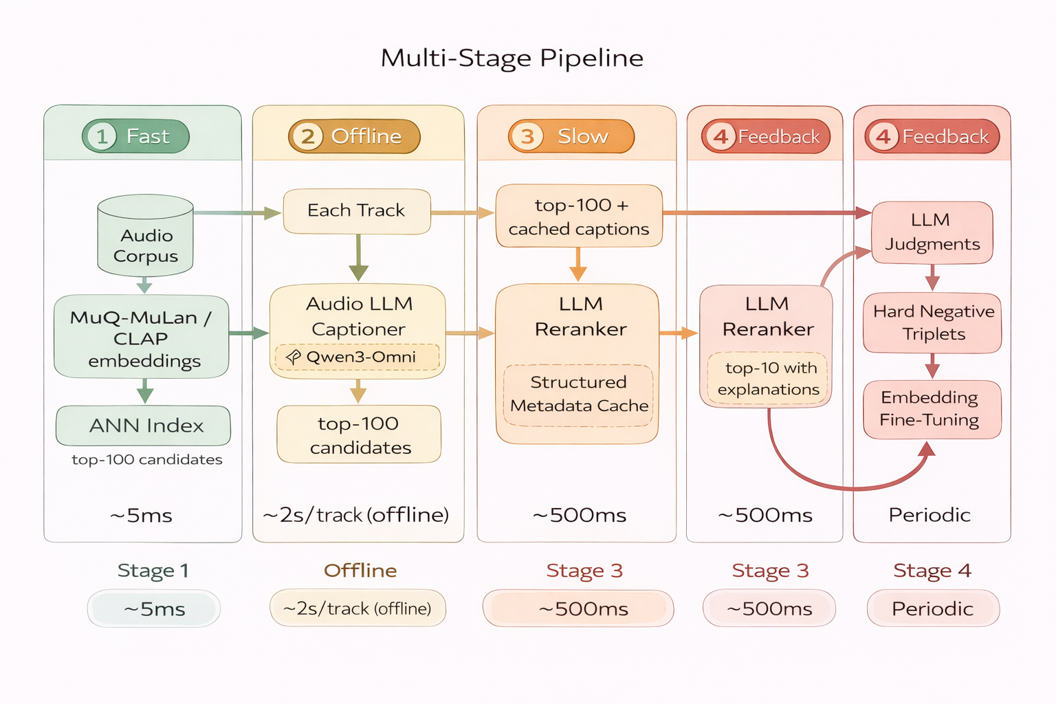
Here we give an example of the possible production architecture for hard negatives mining, which combines components:
Stage 1: Fast Candidate Generation (Online, ~5ms)
Embed the query track with MuQ-MuLan (or CLAP). Retrieve top-$k$ candidates via approximate nearest neighbor (ANN) search. This is purely geometric — cosine similarity in embedding space.
Stage 2: Offline Captioning (Batch, ~2s/track)
Pre-compute structured captions for the entire catalog using an Audio LLM (e.g. Qwen3-Omni or Music Flamingo). Store as metadata: genre, mood, instrumentation, energy, vocal characteristics, lyrical themes, cultural context. This is done once and cached.
Stage 3: LLM Reranking (Online, ~500ms)
Feed the top-$k$ candidates’ cached captions + the query context into an LLM for reranking. The LLM reasons over text descriptions to select and explain the most relevant tracks. No audio processing at serving time — only text reasoning.
Stage 4: Feedback Loop (Periodic, Offline)
Use LLM judgments to mine hard negatives. Fine-tune the embedding model. Deploy the improved embeddings. Repeat.
| Operation | Compute | Frequency | Latency |
|---|---|---|---|
| Embedding inference | Low | Per new track | ~50ms |
| ANN retrieval | Very low | Per query | ~5ms |
| Audio LLM captioning | High | Once per track (offline) | ~2s |
| LLM text reranking | Medium | Per query (top-k only) | ~500ms |
| Hard negative mining + fine-tuning | High | Periodic batch | Hours |
Design principle: keep expensive steps offline; limit online LLM calls to small candidate sets over cached text.
Demo Resources and Experiments
There are nice demo resources, curated by the model’s authors:
Live demo resources:
- Qwen3-Omni Captioner: https://huggingface.co/spaces/Qwen/Qwen3-Omni-Captioner-Demo
- Music Flamingo: https://huggingface.co/spaces/nvidia/music-flamingo
- MuQ-MuLan model: https://huggingface.co/OpenMuQ/MuQ-MuLan-large
But let’s test models ourselves. We deployed all models locally on our infrastructure with VLLM. So lets take some audio tracks (well nice perk of working in music recommendations field is an access to tracks) and test what captions we can get and is the relevance assessment is good and.
Comparing Captioning Models
So lets compare captioning ability of 2 models: Qwen3-Omni Captioner and Qwen 2 Audio. We will use 2 tracks from different genre:
- Nirvana - In Bloom
- Король и Шут - Ели Мясо Мужики (Russian classical rock)
Also we utilize powerful textual LLM (Qwen 3.5 35B-A3B) to extract useful metadata from resulting descriptions.
Qwen3-Omni Captioner
As this model’s prompt is fixed, we can directly deploy and inference it as is. We observed that the model output has a stable structure with physical properties of music, meaning and narrative context. This gives us enough information to extract structured metadata.
| Property | Observation |
|---|---|
| Caption structure | Stable |
| Production details | Present |
| Instrument detection | Accurate |
| Vocal analysis | Detailed |
| Narrative context | Present |
| Stability | High |
The model consistently describes:
- instrumentation
- rhythm section
- vocal delivery
- production aesthetics
- narrative meaning
This makes it very suitable for structured metadata extraction.
Nirvana - In Bloom
The caption includes detailed analysis of:
| Feature | Example extracted |
|---|---|
| Instrumentation | distorted guitars, bass, drum kit |
| Production | compressed mix, stereo width |
| Energy | loud, aggressive |
| Vocals | strained tenor delivery |
| Genre context | grunge / alternative rock |
Extracted metadata:
| |
Король и Шут - Ели Мясо Мужики
The caption correctly captures:
| Feature | Description |
|---|---|
| Vocal style | gravelly theatrical storytelling |
| Instrumentation | distorted guitars + rhythm section |
| Production | lo-fi analog punk aesthetic |
| Lyrics theme | dark humorous storytelling |
| Structure | narrative verses + explosive choruses |
Extracted metadata:
| |
Qwen2 Audio
For this model we used a custom prompt forcing structured perceptual description.
Despite the prompt constraints, the model shows strong instability.
| Issue | Example |
|---|---|
| Ignoring prompt instructions | missing sections |
| Incorrect genre | pop instead of punk |
| Hallucinated theory | chord progressions |
| Short outputs | 1–2 sentences only |
| Language artifacts | “俄语-speaking environment” |
Caption (Nirvana - In Bloom)
Example output:
- hallucinated chord progression
- missing vocal detection
- extremely short description
Extracted metadata:
| |
This misses most perceptual information.
Король и Шут - Ели Мясо Мужики
The model misclassified the track entirely:
| Predicted | Actual |
|---|---|
| Pop | Punk rock |
| Slow tempo | Fast |
| Synth instruments | Distorted guitars |
Metadata becomes unusable for similarity analysis.
Comparison and MuQ-Mulan Embeddings
To evaluate caption quality we computed similarities using MuQ-Mulan embeddings.
Measured similarities:
- caption ↔ track
- summarized description ↔ track
- caption ↔ summarized description
Higher similarity indicates better semantic alignment.
Comparison (Nirvana - In Bloom)
| Model | Caption ↔ Track | Summary ↔ Track | Caption ↔ Summary |
|---|---|---|---|
| Qwen2 Audio | 0.293 | 0.233 | 0.352 |
| Qwen3 Captioner | 0.3909 | 0.284 | 0.438 |
Observations:
- Qwen3 captions align significantly better with audio
- summarization causes some information loss
- Qwen2 still provides a reasonable baseline
Comparison (Король и Шут - Ели Мясо Мужики)
| Model | Caption ↔ Track | Summary ↔ Track | Caption ↔ Summary |
|---|---|---|---|
| Qwen2 Audio | 0.01 | 0.24 | 0.65 |
| Qwen3 Captioner | 0.3614 | 0.284 | 0.438 |
Observation: Qwen2 caption embedding is nearly unrelated to the track.
Using Relevance Judge
We use an LLM-based music similarity judge based on core perceptual dimensions.
Core similarity dimensions:
| Dimension |
|---|
| Genre family |
| Production style |
| Timbre |
| Vocal role |
| Vocal delivery |
Secondary dimensions:
- tempo
- energy
- mood
- usage context
Secondary dimensions alone cannot justify similarity.
Qwen3 – Omni Captioner + LLM judge
Result: SIMILAR
Reason:
| Shared attributes |
|---|
| distorted guitar band sound |
| high energy |
| fast tempo |
| aggressive male vocals |
| punk / alternative rock lineage |
Differences:
| Differences |
|---|
| language |
| subgenre |
| vocal delivery style |
This aligns well with human musical intuition.
Qwen 2 Audio + LLM judge
Result: NOT_SIMILAR
Reason: One track was misclassified as slow synth pop which breaks similarity evaluation.
Conclusion
| Criterion | Best Model |
|---|---|
| Caption richness | Qwen3-Omni |
| Perceptual accuracy | Qwen3-Omni |
| Embedding alignment | Qwen3-Omni |
| Stability | Qwen3-Omni |
Qwen3-Omni Captioner is the better teacher model for distillation.
It produces captions that:
- capture perceptual characteristics of audio
- align well with audio embeddings
- enable reliable metadata extraction
- support similarity reasoning
Recommended Pipeline

Pipeline Flow:
- Audio Track → Input music file
- Qwen3-Omni Captioner → Generate rich text description
- Metadata Extraction LLM → Structure into schema fields
- TrackSummary Schema → Structured metadata object
- Embedding (MuQ-MuLan) → Generate vector representation
- Similarity / RAG / Playlist Systems → Power recommendations
Conclusion
The path from acoustic similarity to perceptual relevance cannot be walked by embeddings alone. Foundation models — MusicFM for acoustic structure, CLAP for language-grounded retrieval, MuQ-MuLan for music-aware joint embeddings — provide the fast, scalable backbone. But they compress music into static vectors where context, intent, and meaning are lost.
Audio LLMs restore what embeddings discard: compositional reasoning, contextual judgment, and natural language explainability. The hybrid architecture — fast embedding retrieval + offline captioning + slow LLM reranking + hard negative feedback — combines the strengths of both paradigms while respecting production latency constraints.
The most promising direction is the feedback loop: using LLM judgments to mine hard negatives that progressively align the embedding space with human-perceived relevance. Each cycle makes the fast path smarter, reducing dependence on the slow path over time.
Music understanding is moving from “what does it sound like?” to “what does it mean, to whom, and why?”
In future articles we will deep dive into audio LLMs architectures and perform some experiments on the suitability of these LLMs for improving recommendations and other real-life production needs.
References
- Elizalde, B., et al. (2022). CLAP: Learning Audio Concepts From Natural Language Supervision. arXiv:2206.04769. https://arxiv.org/abs/2206.04769
- Won, M., Hung, Y., & Le, D. (2023). A Foundation Model for Music Informatics. arXiv:2311.03318. https://arxiv.org/abs/2311.03318
- Ghosh, S., et al. (2025). Music Flamingo: Scaling Music Understanding in Audio Language Models. arXiv:2511.10289. https://arxiv.org/abs/2511.10289
- Qwen Team. (2025). Qwen3-Omni Technical Report. arXiv:2509.17765. https://arxiv.org/abs/2509.17765
- Gong, Y., et al. (2024). Listen, Think, and Understand. ICLR 2024. arXiv:2305.10790. https://arxiv.org/abs/2305.10790
- Audio Flamingo 3. (2025). arXiv:2507.08128. https://arxiv.org/abs/2507.08128
- Zhu, H., et al. (2025). MuQ: Self-Supervised Music Representation Learning with Mel Residual Vector Quantization. arXiv:2501.01108. https://arxiv.org/abs/2501.01108
- Perceptually-Aligned Music Similarity. (2026). arXiv:2601.19109. https://arxiv.org/abs/2601.19109
- Mei, M. J., et al. (2025). Semantic IDs for Music Recommendation. arXiv:2507.18800. https://arxiv.org/abs/2507.18800
- Chu, Y., et al. (2024). Qwen2-Audio Technical Report. arXiv:2407.10759. https://arxiv.org/abs/2407.10759
- Li, X., et al. (2025). Kimi-Audio: A Unified Audio Foundation Model for Understanding, Generation, and Conversation. arXiv:2504.18425. https://arxiv.org/abs/2504.18425